Introduction
Searching through an unsorted database is one of the most fundamental problems in computer science. With a classical computer, finding a specific item among N entries requires checking N/2 items on average, and N in the worst case. Quantum computers change this picture entirely—they can solve the same problem in O(√N) time.
This is Grover’s Algorithm, proposed by Lov Grover in 1996.
Classical vs Quantum Search
The Classical Approach
Imagine searching for a specific phone number in an unsorted phone book. A classical computer has no choice but to check entries one by one:
def classical_search(database, target):
    for i, item in enumerate(database):
        if item == target:
            return i
return -1 # Not found- Time complexity: O(N)
- Best case: 1 check (lucky guess)
- Average: N/2 checks
- Worst case: N checks
The Quantum Approach
Grover’s Algorithm uses quantum superposition and amplitude amplification to dramatically reduce this number:
- Time complexity: O(√N)
- Required iterations: roughly π√N/4
For N=1,000,000 items:
- Classical: 500,000 checks on average
- Quantum: about 785 checks (√1,000,000 ≈ 1,000)
This quadratic speedup might not sound as dramatic as exponential speedups, but it applies to a broad class of problems.
Core Idea
Grover’s Algorithm repeats two operations:
- Oracle: Mark the target state
- Diffusion Operator: Amplify the marked state’s amplitude
Geometrically, each iteration rotates the quantum state toward the target.
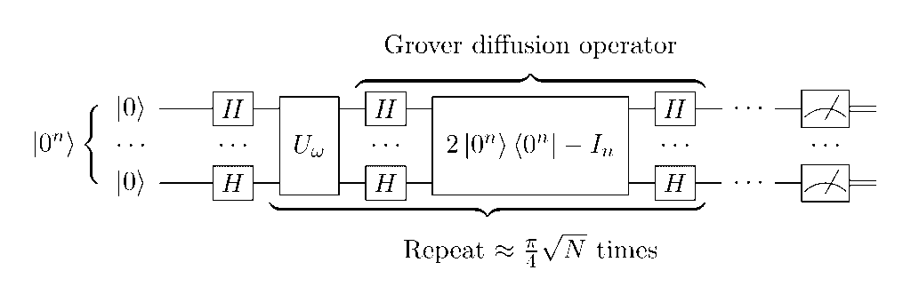
Step 1: Initialize with Uniform Superposition
Start by putting all possible states into equal superposition:
$$|\psi_0\rangle = \frac{1}{\sqrt{N}} \sum_{x=0}^{N-1} |x\rangle$$
This comes from applying Hadamard gates to all qubits.
Step 2: Oracle Operation
The oracle $O$ flips the phase of the target state $|w\rangle$:
$$O|x\rangle = \begin{cases} -|x\rangle & \text{if } x = w \ |x\rangle & \text{if } x \neq w \end{cases}$$
Mathematically:
$$O = \mathbf{I} – 2|w\rangle\langle w|$$
The oracle is essentially a quantum circuit that can recognize the target.
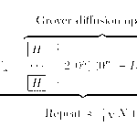
Step 3: Diffusion Operator
This performs “inversion about average”:
$$D = 2|\psi_0\rangle\langle\psi_0| – \mathbf{I}$$
The operation:
- Calculates the average amplitude across all states
- Reflects each state’s amplitude about this average
The target state’s amplitude grows while others shrink.
Step 4: Grover Iteration
One Grover iteration $G$ combines both:
$$G = D \cdot O$$
After about $\frac{\pi}{4}\sqrt{N}$ iterations, the target state has near-unit probability.
Geometric Picture
Grover’s Algorithm can be visualized in 2D space:
- Target state: $|w\rangle$
- Superposition of all other states: $|s’\rangle = \frac{1}{\sqrt{N-1}} \sum_{x \neq w} |x\rangle$
The initial state $|\psi_0\rangle$ is a superposition of these two:
$$|\psi_0\rangle = \sin\theta |w\rangle + \cos\theta |s’\rangle$$
where $\sin\theta = \frac{1}{\sqrt{N}}$.
Each Grover iteration rotates the state by roughly $2\theta$ toward the target. So:
- Number of rotations needed: $\frac{\pi/2}{2\theta} \approx \frac{\pi}{4\sin\theta} \approx \frac{\pi}{4}\sqrt{N}$
Qiskit Implementation: Searching 4 Items
Let’s implement Grover’s Algorithm for a simple case—finding $|11\rangle$ among 4 items (2 qubits).
from qiskit import QuantumCircuit, QuantumRegister, ClassicalRegister
from qiskit_aer import AerSimulator
from qiskit.visualization import plot_histogram
import numpy as np
# 2 qubits = 4 items (00, 01, 10, 11)
n = 2
qr = QuantumRegister(n, 'q')
cr = ClassicalRegister(n, 'c')
qc = QuantumCircuit(qr, cr)
# Step 1: Initialize uniform superposition
qc.h(qr) # Hadamard on all qubits
qc.barrier()
# Step 2: Oracle - mark |11>
# Use controlled-Z to flip phase only for |11>
qc.cz(0, 1)
qc.barrier()
# Step 3: Diffusion Operator
# 3-1. H gates
qc.h(qr)
# 3-2. X gates (flip 0→1)
qc.x(qr)
# 3-3. Multi-controlled Z
qc.h(1)
qc.cx(0, 1)
qc.h(1)
# 3-4. X gates (flip back)
qc.x(qr)
# 3-5. H gates
qc.h(qr)
qc.barrier()
# Step 4: Measure
qc.measure(qr, cr)
# Run
simulator = AerSimulator()
result = simulator.run(qc, shots=1024).result()
counts = result.get_counts()
print("Measurement results:")
print(counts)
# Expected: {'11': ~1024} (nearly 100% probability for 11)Code Breakdown
- Initialize:
qc.h(qr)creates equal superposition of all states - Oracle:
qc.cz(0, 1)flips phase only for |11> - Diffusion:
- H → X → Multi-CZ → X → H sequence
- Implements “inversion about average”
- Measure: Results show ~100% probability for |11>
Analysis
With N=4 items, $\sqrt{N} = 2$. Theory predicts:
- Grover iterations needed: $\frac{\pi}{4} \times 2 \approx 1.57$ ≈ 1
Our code performs exactly 1 iteration and finds the target with near-certainty.
Scaling Up: 8 Items (3 qubits)
With 3 qubits, we can search among 8 items. To find |101>:
n = 3
# ... (initialization code)

# Oracle for |101>
qc.x(1)  # Flip middle qubit to target 0
qc.h(2)
qc.ccx(0, 1, 2)  # Toffoli gate
qc.h(2)
qc.x(1)  # Flip back

# ... (Diffusion operator)Required iterations: $\frac{\pi}{4}\sqrt{8} \approx 2.2$ ≈ 2
Applications and Limitations
Where It’s Useful
- Database search: Unstructured data lookup
- Optimization: Finding solutions in combinatorial spaces
- Cryptanalysis: Speeding up brute-force attacks (security concern!)
- SAT problems: Boolean satisfiability
Practical Limitations
Grover’s Algorithm faces several constraints:
- Oracle cost: Building the oracle can be complex
- Quadratic speedup: Modest compared to Shor’s exponential advantage
- NISQ-era constraints:
- Limited qubits ($n$ qubits → $2^n$ items)
- Decoherence errors
- Error accumulation over many iterations
4. Optimality: Proven to be optimal—no quantum algorithm can do better
When Does It Actually Help?
Grover’s Algorithm is useful when:
$$T_{\text{quantum}} < T_{\text{classical}}$$
Which means:
$$T_{\text{oracle}} \times \sqrt{N} < T_{\text{classical check}} \times N$$
If the oracle is too expensive to build, quantum loses its advantage.
Example with N=1,000,000:
- Classical: 500,000 checks
- Quantum: ~785 oracle calls
If the oracle is 100× slower than classical check? → Quantum still wins (~6× faster)
If the oracle is 1000× slower than classical check? → Classical is better
References
- Grover, L. K. (1996). A fast quantum mechanical algorithm for database search. Proceedings of the 28th Annual ACM Symposium on Theory of Computing, 212-219.
- Nielsen, M. A., & Chuang, I. L. (2010). Quantum Computation and Quantum Information. Cambridge University Press. (Chapter 6: Quantum search algorithms)
- IBM Qiskit Documentation. “Grover’s Algorithm.” https://qiskit.org/textbook/ch-algorithms/grover.html
- Boyer, M., Brassard, G., Høyer, P., & Tapp, A. (1998). Tight bounds on quantum searching. Fortschritte der Physik, 46(4-5), 493-505.
- Zalka, C. (1999). Grover’s quantum searching algorithm is optimal. Physical Review A, 60(4), 2746.
Coming next: VQE and QAOA – Practical quantum algorithms for the NISQ era
Related posts: