Quantum States and MeasuremenT-Understanding how quantum systems represent and reveal information-
1. Classical vs Quantum Descriptions
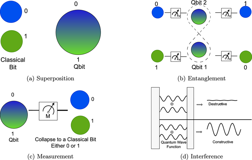
In classical physics, the state of a system is a definite configuration—position, velocity, or spin direction can be known simultaneously.
In contrast, a quantum state encodes probabilities and superpositions of all possible outcomes.
A single qubit, for example, can exist in
$$ |\psi\rangle = \alpha |0\rangle + \beta |1\rangle, $$
where \(\alpha\) and \(\beta\) are complex amplitudes satisfying \(|\alpha|^2 + |\beta|^2 = 1\).
Unlike classical bits, measurement collapses this state to either \(|0\rangle\) or \(|1\rangle\) probabilistically, not deterministically.
2. Quantum State Representation
Quantum states live in a Hilbert space, a complex vector space equipped with an inner product.
Each physical system corresponds to a normalized vector \(|\psi\rangle\).
Pure vs Mixed States
- Pure state: Fully known vector \(|\psi\rangle\)
- Mixed state: Statistical ensemble of pure states, represented by a density operator \(\rho\)
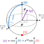
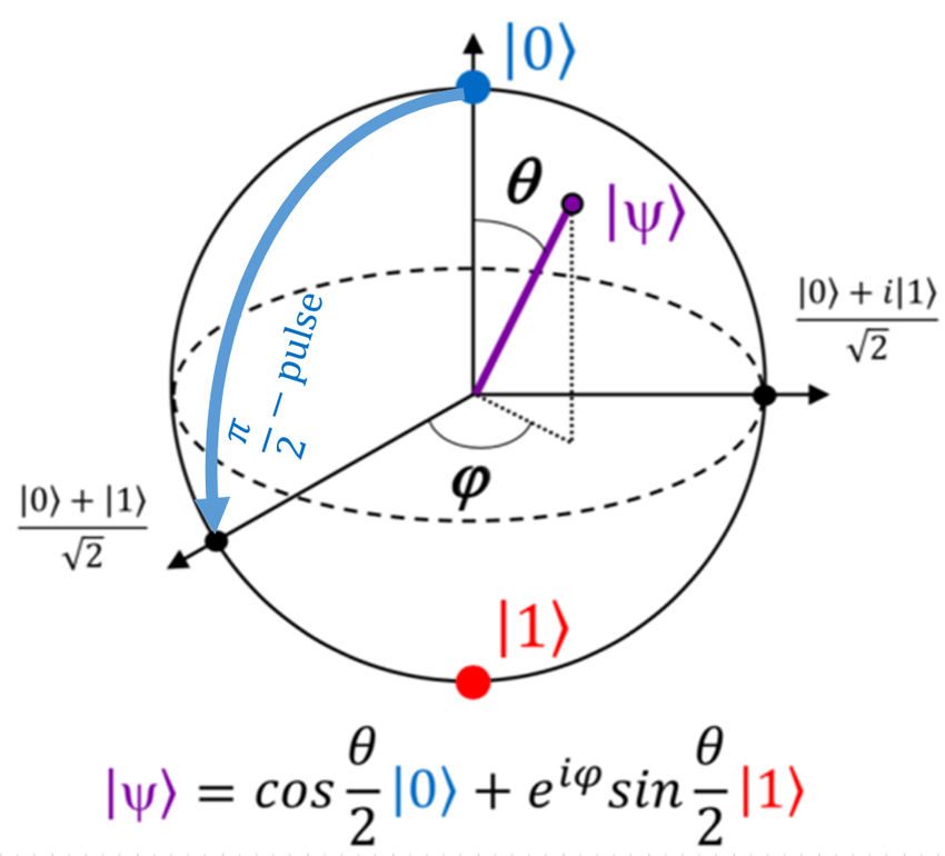
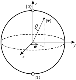
Any single-qubit pure state can be rewritten as
$$ |\psi\rangle = \cos\frac{\theta}{2}|0\rangle + e^{i\phi}\sin\frac{\theta}{2}|1\rangle, $$
which maps to a point on the unit sphere with angles \((\theta, \phi)\).
3. Measurement in Quantum Mechanics
Measurement is described by a set of Hermitian operators called observables.
Each observable \(\hat{A}\) has eigenstates \(|a_i\rangle\) and real eigenvalues \(a_i\).
The Born rule defines measurement probabilities:
$$ P(a_i) = |\langle a_i | \psi \rangle|^2. $$
After measurement, the system collapses to \(|a_i\rangle\).
$$ X = \begin{pmatrix} 0 & 1 \ 1 & 0 \end{pmatrix} $$
If the qubit is in \(|0\rangle\), measuring \(X\) can yield either eigenstate
$$ |+\rangle = \frac{1}{\sqrt{2}}(|0\rangle + |1\rangle), \quad |-\rangle = \frac{1}{\sqrt{2}}(|0\rangle – |1\rangle). $$
4. Density Matrix Formalism
For mixed or entangled systems, we use the density operator
$$ \rho = \sum_i p_i |\psi_i\rangle\langle\psi_i|, $$
where \(p_i\) are classical probabilities.
The expectation value of an observable \(A\) is
$$ \langle A \rangle = \mathrm{Tr}(\rho A). $$
When considering subsystems, we obtain the reduced density matrix via partial trace—this operation is central in describing entanglement and decoherence.
5. From Theory to Experiment
In quantum hardware, measurement corresponds to projective readout in the computational basis.
In IBM Qiskit, for instance:
from qiskit import QuantumCircuit
qc = QuantumCircuit(1,1)
qc.h(0)
qc.measure(0,0)Here, the \(H\) (Hadamard) gate creates superposition, and measure() collapses the state to 0 or 1 with equal probability.
Physical devices approximate ideal projective measurements but include noise and decoherence, making density-matrix simulation essential in realistic modeling.
6. Summary and Outlook
Quantum states encode probabilistic information in complex amplitudes.
Measurement extracts classical information according to the Born rule, fundamentally altering the system.
This transition from coherent evolution to measurement underpins all quantum algorithms.
Next in the Quantum Computing Fundamentals series: Quantum Gates and Circuits, where we explore how unitary operations manipulate these states before measurement.
References
- M. A. Nielsen and I. L. Chuang, Quantum Computation and Quantum Information, Cambridge Univ. Press (2010).
- J. Preskill, Lecture Notes on Quantum Computation (Caltech).
- IBM Quantum Documentation: https://quantum.ibm.com
- D. Griffiths, Introduction to Quantum Mechanics, 2nd ed. Pearson (2016).