Quantum Circuits Fundamentals: Building Blocks of Quantum Computing
In our previous posts exploring Bell states and quantum entanglement, we used specific quantum gates like the Hadamard (H) and CNOT gates to create and manipulate quantum states. These gates are the fundamental building blocks of all quantum circuits, much like how logic gates form the foundation of classical computing. Understanding quantum circuits fundamentals is essential for anyone serious about quantum computing, as every quantum algorithm and protocol is ultimately constructed from these basic elements.
While our Bell state experiments gave us a glimpse into quantum gate operations, we barely scratched the surface of what’s possible with quantum circuits. Today, we’ll dive deeper into the mathematical structure and practical implementation of quantum gates, exploring how they transform quantum states and why certain combinations produce the remarkable phenomena we observe in quantum computing.
The Mathematical Foundation of Quantum Gates
Quantum gates are unitary operators that act on quantum states in a reversible manner. Unlike classical logic gates that operate on definite bit values, quantum gates manipulate probability amplitudes in a complex vector space. This fundamental difference is what gives quantum computing its power.
Every quantum gate can be represented as a unitary matrix U, where U†U = I (the identity matrix). This constraint ensures that quantum evolution preserves probability – the total probability of measuring any outcome must always equal 1. When we apply a gate to a quantum state |ψ⟩, we’re performing a matrix multiplication: |ψ’⟩ = U|ψ⟩.
The requirement for unitarity means that quantum gates are always reversible. For every quantum gate U, there exists an inverse gate U† that undoes its operation. This reversibility is a fundamental principle of quantum mechanics and distinguishes quantum computation from classical computation, where many operations (like the classical AND gate) are irreversible.
Single-Qubit Gates: The Basic Transformations
Pauli Gates: The Foundation
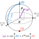
The Pauli gates form the cornerstone of single-qubit operations. Named after physicist Wolfgang Pauli, these gates perform specific rotations on the Bloch sphere representation of a qubit.
The Pauli-X gate (also called the NOT gate) performs a bit flip operation:
$$X = \begin{pmatrix} 0 & 1 \\ 1 & 0 \end{pmatrix}$$
When applied to the basis states, X|0⟩ = |1⟩ and X|1⟩ = |0⟩. On the Bloch sphere, this represents a 180° rotation around the X-axis. In classical terms, it’s equivalent to a NOT operation, but unlike classical NOT gates, the Pauli-X can operate on superposition states, flipping the amplitudes between |0⟩ and |1⟩ components.
The Pauli-Y gate combines both bit flip and phase flip operations:
$$Y = \begin{pmatrix} 0 & -i \\ i & 0 \end{pmatrix}$$
This gate performs a 180° rotation around the Y-axis on the Bloch sphere. It’s particularly useful in quantum algorithms that require both amplitude and phase manipulation simultaneously.
The Pauli-Z gate performs a phase flip without affecting the computational basis probabilities:
$$Z = \begin{pmatrix} 1 & 0 \\ 0 & -1 \end{pmatrix}$$
This gate leaves |0⟩ unchanged but adds a minus sign to |1⟩: Z|0⟩ = |0⟩ and Z|1⟩ = -|1⟩. While this change is invisible when measuring in the computational basis, it has profound effects on interference patterns and is crucial for many quantum algorithms.
Hadamard Gate: Creating Superposition
The Hadamard gate is perhaps the most important single-qubit gate for quantum computing:
$$H = \frac{1}{\sqrt{2}}\begin{pmatrix} 1 & 1 \\ 1 & -1 \end{pmatrix}$$
This gate creates superposition states from computational basis states. Applying H to |0⟩ produces the state (|0⟩ + |1⟩)/√2, an equal superposition of both basis states. The Hadamard gate is its own inverse: applying it twice returns the original state (H² = I).
The power of the Hadamard gate becomes apparent when we consider its effect on measurement. A qubit in the |+⟩ = H|0⟩ state has a 50% probability of measuring |0⟩ or |1⟩, but this randomness is fundamentally different from classical randomness – it arises from quantum superposition rather than lack of information.
Let’s implement a simple example to see these gates in action:
from qiskit import QuantumCircuit, transpile
from qiskit_aer import AerSimulator
from qiskit.visualization import plot_histogram
import numpy as np

# Create a circuit to test single-qubit gates
def test_single_qubit_gates():
    # Test Pauli-X gate
    qc_x = QuantumCircuit(1, 1)
    qc_x.x(0)  # Apply X gate
    qc_x.measure(0, 0)

    # Test Hadamard gate
    qc_h = QuantumCircuit(1, 1)
    qc_h.h(0)  # Apply H gate
    qc_h.measure(0, 0)

    # Test X then H combination
    qc_xh = QuantumCircuit(1, 1)
    qc_xh.x(0)   # First apply X
    qc_xh.h(0)   # Then apply H
    qc_xh.measure(0, 0)

    # Simulate all circuits
    simulator = AerSimulator()
    shots = 1000

    results = {}
    for name, circuit in [("X gate", qc_x), ("H gate", qc_h), ("X+H", qc_xh)]:
        job = simulator.run(transpile(circuit, simulator), shots=shots)
        counts = job.result().get_counts()
        results[name] = counts
        print(f"{name}: {counts}")

    return results

# Run the test
gate_results = test_single_qubit_gates()
Phase Gates: Precise Phase Control
Beyond the Pauli gates, we have phase gates that provide more precise control over quantum phases. The S gate (also called the phase gate) adds a phase of i to the |1⟩ state:
$$S = \begin{pmatrix} 1 & 0 \\ 0 & i \end{pmatrix}$$
The T gate adds a phase of \(e^{iπ/4} \) to the |1⟩ state:
$$T = \begin{pmatrix} 1 & 0 \\ 0 & e^{i\pi/4} \end{pmatrix}$$
These phase gates are particularly important because they, together with the Hadamard gate, form a universal set for single-qubit operations. Any single-qubit unitary can be decomposed into a sequence of H, S, and T gates.
Multi-Qubit Gates: Creating Entanglement
While single-qubit gates can create superposition, they cannot create entanglement between qubits. For that, we need multi-qubit gates that operate on two or more qubits simultaneously.
CNOT Gate: The Fundamental Two-Qubit Operation
The Controlled-NOT (CNOT) gate is the most important two-qubit gate. It performs a NOT operation on the target qubit if and only if the control qubit is in state |1⟩:
$$\text{CNOT} = \begin{pmatrix} 1 & 0 & 0 & 0 \\ 0 & 1 & 0 & 0 \\ 0 & 0 & 0 & 1 \\ 0 & 0 & 1 & 0 \end{pmatrix}$$
The CNOT gate operates on the computational basis states as follows:
- |00⟩ → |00⟩ (control=0, target unchanged)
- |01⟩ → |01⟩ (control=0, target unchanged)
- |10⟩ → |11⟩ (control=1, target flipped)
- |11⟩ → |10⟩ (control=1, target flipped)
The true power of CNOT becomes apparent when the control qubit is in superposition. Starting with the state H|0⟩⊗|0⟩ = (|0⟩ + |1⟩)⊗|0⟩/√2 = (|00⟩ + |10⟩)/√2, applying CNOT produces (|00⟩ + |11⟩)/√2 – the Bell state we’ve encountered before.
Let’s implement a circuit that demonstrates CNOT’s entangling power:
def demonstrate_cnot_entanglement():
    # Create Bell state using H + CNOT
    qc = QuantumCircuit(2, 2)

    # Apply Hadamard to first qubit (creates superposition)
    qc.h(0)

    # Apply CNOT with qubit 0 as control, qubit 1 as target
    qc.cx(0, 1)

    # Add measurements
    qc.measure_all()

    # Simulate
    simulator = AerSimulator()
    job = simulator.run(transpile(qc, simulator), shots=1000)
    counts = job.result().get_counts()

    print("Bell state measurement results:")
    print(counts)

    # Expected: roughly 50% |00⟩ and 50% |11⟩, no |01⟩ or |10⟩
    return qc, counts

bell_circuit, bell_counts = demonstrate_cnot_entanglement()
print(f"Circuit depth: {bell_circuit.depth()}")
Toffoli Gate: Quantum AND Operation
The Toffoli gate (also called the CCX or controlled-controlled-X gate) is a three-qubit gate that flips the target qubit if and only if both control qubits are in state |1⟩. This gate is particularly interesting because it’s universal for classical computation – any classical logic circuit can be built using only Toffoli gates.
The Toffoli gate provides a direct bridge between classical and quantum computing. It performs the operation |a,b,c⟩ → |a,b,c⊕(a∧b)⟩, where ⊕ is XOR and ∧ is AND. When the target qubit starts in |0⟩, the output becomes |a,b,a∧b⟩, implementing classical AND logic.
def demonstrate_toffoli_and():
    # Test all possible inputs for classical AND operation
    results = {}

    for a in [0, 1]:
        for b in [0, 1]:
            qc = QuantumCircuit(3, 3)

            # Prepare input state |a,b,0⟩
            if a == 1:
                qc.x(0)
            if b == 1:
                qc.x(1)
            # Qubit 2 starts in |0⟩

            # Apply Toffoli gate
            qc.ccx(0, 1, 2)  # Control qubits 0,1; target qubit 2

            # Measure
            qc.measure_all()

            # Simulate
            simulator = AerSimulator()
            job = simulator.run(transpile(qc, simulator), shots=100)
            counts = job.result().get_counts()

            # Extract most likely result
            result_state = max(counts.keys(), key=counts.get)
            output_c = int(result_state[0])  # Rightmost bit (qubit 2)

            results[(a,b)] = output_c
            print(f"AND({a},{b}) = {output_c}")

    return results

and_results = demonstrate_toffoli_and()
Circuit Design and Optimization
IBM Quantum Hardware Constraints
Real quantum computers impose significant constraints on circuit design. IBM’s quantum processors use a “heavy-hex” topology, where qubits are arranged in a hexagonal lattice with additional qubits in the center. This topology determines which qubits can directly interact through two-qubit gates.
When designing circuits for real hardware, we must consider:
Connectivity constraints: Two-qubit gates can only be applied between physically connected qubits. If your algorithm requires a CNOT between non-adjacent qubits, the quantum compiler must insert SWAP gates to move the quantum information, increasing circuit depth and error rates.
Gate errors: Each gate operation has an associated error rate. Single-qubit gates typically have error rates around 0.1%, while two-qubit gates have higher error rates around 1%. Minimizing the number of two-qubit gates is crucial for maintaining fidelity.
Decoherence time: Quantum states decay over time due to environmental interaction. The coherence time (T1 and T2 times) limits how long we can maintain quantum information, constraining the maximum circuit depth.
Circuit Depth Optimization
Circuit depth – the number of sequential gate operations – is a critical metric for quantum circuits. Deeper circuits are more susceptible to errors and decoherence. Modern quantum compilers employ various optimization techniques:
Gate cancellation: Consecutive inverse gates (like H-H or X-X) cancel out and can be removed.
Gate commutation: Gates that commute can be reordered to reduce depth. For example, Z gates commute with other Z gates and with measurements.
Template matching: Common gate sequences can be replaced with more efficient equivalents.
Let’s examine how circuit optimization affects a simple algorithm:
def compare_circuit_optimization():
    # Unoptimized circuit: create GHZ state naively
    qc_unopt = QuantumCircuit(4)
    qc_unopt.h(0)
    for i in range(1, 4):
        qc_unopt.cx(0, i)

    # Optimized circuit: reduce depth using parallel operations
    qc_opt = QuantumCircuit(4)
    qc_opt.h(0)
    # Apply CNOT gates in parallel where possible
    qc_opt.cx(0, 1)
    qc_opt.cx(0, 2)
    qc_opt.cx(0, 3)

    # Another optimization: chain CNOTs
    qc_chain = QuantumCircuit(4)
    qc_chain.h(0)
    qc_chain.cx(0, 1)
    qc_chain.cx(1, 2)
    qc_chain.cx(2, 3)

    circuits = [
        ("Unoptimized", qc_unopt),
        ("Parallel CNOTs", qc_opt),
        ("Chained CNOTs", qc_chain)
    ]

    for name, circuit in circuits:
        print(f"{name}: Depth = {circuit.depth()}, Gates = {sum(circuit.count_ops().values())}")

    return circuits

optimization_comparison = compare_circuit_optimization()
Advanced Multi-Qubit States
GHZ States: Maximum Entanglement
The Greenberger-Horne-Zeilinger (GHZ) states extend the concept of Bell states to multiple qubits. The three-qubit GHZ state is:
$$|GHZ_3⟩ = \frac{1}{\sqrt{2}}(|000⟩ + |111⟩)$$
GHZ states exhibit even more dramatic non-classical correlations than Bell states. They’re maximally entangled states where measuring any subset of qubits immediately determines the measurement outcomes of all remaining qubits.
W States: Distributed Entanglement
W states represent a different type of multi-qubit entanglement:
$$|W_3⟩ = \frac{1}{\sqrt{3}}(|001⟩ + |010⟩ + |100⟩)$$
Unlike GHZ states, W states maintain some entanglement even when one qubit is lost or measured. This robustness makes them valuable for certain quantum communication protocols.
def create_advanced_multiparty_states():
    # Create 3-qubit GHZ state
    def create_ghz_state():
        qc = QuantumCircuit(3, 3)
        qc.h(0)           # Create superposition
        qc.cx(0, 1)       # Entangle qubits 0 and 1
        qc.cx(0, 2)       # Entangle qubit 0 with 2
        return qc

    # Create 3-qubit W state (more complex)
    def create_w_state():
        qc = QuantumCircuit(3, 3)
        # W state requires more sophisticated preparation
        qc.ry(2*np.arccos(np.sqrt(2/3)), 0)  # Rotate to correct amplitude
        qc.cx(0, 1)
        qc.x(0)
        qc.ccx(0, 1, 2)
        qc.x(0)
        return qc

    # Test both states
    simulator = AerSimulator()

    for state_name, circuit in [("GHZ", create_ghz_state()), ("W", create_w_state())]:
        # Add measurements
        test_circuit = circuit.copy()
        test_circuit.measure_all()

        # Simulate
        job = simulator.run(transpile(test_circuit, simulator), shots=1000)
        counts = job.result().get_counts()

        print(f"{state_name} state measurement results:")
        for state, count in sorted(counts.items()):
            probability = count / 1000
            print(f"  |{state}⟩: {probability:.3f}")
        print()

    return create_ghz_state(), create_w_state()

ghz_circuit, w_circuit = create_advanced_multiparty_states()
Performance Considerations in Practice
Gate Fidelity and Error Rates
Real quantum gates are imperfect. Gate fidelity measures how closely a real gate operation matches the ideal unitary transformation. Current superconducting quantum computers achieve single-qubit gate fidelities around 99.9% and two-qubit gate fidelities around 99%.
These error rates accumulate quickly in deep circuits. For a circuit with 100 gates, even with 99% fidelity per gate, the overall fidelity drops to approximately 37%. This fundamental limitation drives the current focus on near-term quantum algorithms that use shallow circuits.
Quantum Error Mitigation
Several techniques help mitigate errors without full quantum error correction:
Zero-noise extrapolation: Run the same circuit at different noise levels and extrapolate to the zero-noise limit.
Symmetry verification: Use the symmetries of your problem to detect and partially correct errors.
Readout error mitigation: Calibrate measurement errors and apply corrections in post-processing.
def demonstrate_error_effects():
    # Create a circuit that's sensitive to errors
    qc = QuantumCircuit(2, 2)

    # Create Bell state
    qc.h(0)
    qc.cx(0, 1)

    # Add many identity operations (these accumulate noise on real hardware)
    for _ in range(10):
        qc.i(0)  # Identity gate (should do nothing, but adds noise)
        qc.i(1)

    qc.measure_all()

    # On real hardware, you'd see degradation in Bell state fidelity
    # Here we'll simulate with a noise model
    from qiskit_aer.noise import NoiseModel, depolarizing_error

    # Create a simple noise model
    noise_model = NoiseModel()
    error_rate = 0.01  # 1% error rate
    noise_model.add_all_qubit_quantum_error(depolarizing_error(error_rate, 1), ['i', 'h'])
    noise_model.add_all_qubit_quantum_error(depolarizing_error(error_rate * 2, 2), ['cx'])

    # Run with and without noise
    simulator = AerSimulator()

    # Noiseless simulation
    job_ideal = simulator.run(transpile(qc, simulator), shots=1000)
    counts_ideal = job_ideal.result().get_counts()

    # Noisy simulation
    job_noisy = simulator.run(transpile(qc, simulator), shots=1000, noise_model=noise_model)
    counts_noisy = job_noisy.result().get_counts()

    print("Ideal Bell state:")
    print(counts_ideal)
    print("\nWith noise model:")
    print(counts_noisy)

    return counts_ideal, counts_noisy

ideal_results, noisy_results = demonstrate_error_effects()
Building Intuition: From Gates to Algorithms
Understanding quantum circuits fundamentals provides the foundation for quantum algorithms. Every quantum algorithm, from simple quantum teleportation to complex optimization routines, is ultimately a specific arrangement of these basic gates.
The key insight is that quantum circuits don’t just process information – they sculpt probability amplitudes in a high-dimensional space. Each gate operation rotates, reflects, or otherwise transforms these amplitudes, and the final measurement collapses this carefully crafted probability distribution into classical outcomes.
As we’ve seen, the power of quantum computing emerges from three key properties: superposition (creating multiple computational paths simultaneously), entanglement (correlating qubits in non-classical ways), and interference (amplifying correct answers while canceling wrong ones). Every quantum gate contributes to one or more of these effects.
The circuits we’ve explored today – from simple Pauli operations to complex multi-qubit entangled states – represent the basic vocabulary of quantum computation. In our next posts, we’ll see how these building blocks combine to create quantum algorithms that solve problems intractable for classical computers.
The journey from understanding individual gates to implementing full quantum algorithms requires developing intuition about how quantum information flows through circuits. This intuition, combined with careful attention to real hardware constraints, forms the basis of practical quantum programming.
This post completes our exploration of the basics of quantum information. In the next post, we’ll begin studying quantum algorithms, starting with the Deutsch-Jozsa algorithm – our first example of quantum advantage in action.
References
- Nielsen, M. A., & Chuang, I. L. (2010). Quantum Computation and Quantum Information. Cambridge University Press.
- Mermin, N. D. (2007). Quantum Computer Science. Cambridge University Press.
- IBM Qiskit Documentation. “Quantum Circuits.” https://qiskit.org/documentation/
- Cross, A. W., et al. (2022). “OpenQASM 3: A broader and deeper quantum assembly language.” ACM Transactions on Quantum Computing, 3(3), 1-50.
- Preskill, J. (2018). “Quantum Computing in the NISQ era and beyond.” Quantum, 2, 79.