Bell Theorem Inequality Violation: From EPR Paradox to Quantum Information

When I first encountered the Bell theorem inequality during my quantum mechanics studies, I initially dismissed it as yet another abstract mathematical exercise. However, as I delved deeper into quantum information theory and began implementing entanglement protocols in Qiskit, I realized that Bell’s theorem represents one of the most profound foundational results in modern physics. The violation of Bell inequalities doesn’t merely challenge classical intuition—it provides the mathematical bedrock for quantum information processing technologies and fundamentally constrains any realistic interpretation of quantum mechanics.

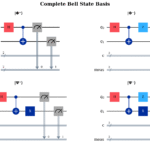
Building upon the mathematical framework of Bell states quantum theory from my previous post, we now examine how these maximally entangled states enable violations of Bell inequalities, thereby providing definitive experimental proof that quantum mechanics cannot be reconciled with local hidden variable theories.

The EPR Paradox: Formalizing the Completeness Problem

The 1935 Einstein-Podolsky-Rosen (EPR) paper presented a rigorous challenge to the completeness of quantum mechanics through what they termed “elements of physical reality.” Their argument, while philosophically motivated, was mathematically precise and established the conceptual foundation for all subsequent work on quantum non-locality.

Formalization of the EPR Argument

Consider a bipartite quantum system prepared in the state:

$$|\psi\rangle = \frac{1}{\sqrt{2}}(|+\rangle_A |!-\rangle_B – |-\rangle_A |+\rangle_B)$$

where \(|±\rangle\) represent eigenstates of the Pauli-Z operator. The EPR argument proceeded through the following logical steps:

1. Reality Criterion: If we can predict with certainty the value of a physical quantity without disturbing the system, then there exists an element of physical reality corresponding to that quantity.
2. Locality Assumption: No real physical influence can propagate faster than light (Einstein causality).
3. Perfect Correlations: Measurement of \(\sigma_z^{(A)}\) on subsystem A yields outcome \( s_A = ±1\) with the measurement of \(\sigma_z^{(B)}\) guaranteed to yield \(s_B = -s_A\).
4. Spatial Separation: If the measurements are spacelike separated, then the measurement on A cannot causally influence the outcome on B.

From these premises, EPR concluded that the spin component of particle B along the z-axis must have possessed a definite value prior to measurement, contradicting the quantum mechanical description where the reduced density matrix \(\rho_B = \text{Tr}_A(|\psi\rangle\langle\psi|) = \frac{1}{2}\mathbf{I}\) indicates maximal mixedness.

“No reasonable definition of reality could be expected to permit this… We are thus forced to conclude that the quantum-mechanical description of physical reality given by wave functions is not complete.” – Einstein, Podolsky, and Rosen (1935)

The EPR argument naturally led to local hidden variable theories, where quantum mechanical probabilities arise from averaging over unknown classical parameters \(\lambda\) distributed according to some measure \(\rho(\lambda)\):

$$P(a,b|x,y) = \int d\lambda , \rho(\lambda) , P_A(a|x,\lambda) , P_B(b|y,\lambda)$$

where \(P_A(a|x,\lambda)\) and \(P_B(b|y,\lambda)\) are deterministic response functions for Alice and Bob respectively.

Bell’s Mathematical Framework: Deriving the Fundamental Inequality

John Stewart Bell’s 1964 breakthrough was to derive experimentally testable consequences of local hidden variable theories that could be compared against quantum mechanical predictions. His approach was to establish mathematical constraints that any local realistic theory must satisfy.

The Original Bell Inequality Derivation

Consider measurement settings characterized by unit vectors \(\vec{a}\) and \(\vec{b}\) for Alice and Bob respectively, with outcomes \(A(\vec{a},\lambda) = ±1\) and \(B(\vec{b},\lambda) = ±1\). The correlation function is:

$$E(\vec{a},\vec{b}) = \int d\lambda , \rho(\lambda) , A(\vec{a},\lambda) , B(\vec{b},\lambda)$$

Bell’s original inequality can be derived by considering three measurement directions \(\vec{a}\), \(\vec{b}\), and \(\vec{c}\):

$$|E(\vec{a},\vec{b}) – E(\vec{a},\vec{c})| \leq 1 + E(\vec{b},\vec{c})$$

However, this form proved difficult to test experimentally due to the requirement for perfect efficiency.

The CHSH Inequality: A More Practical Formulation

Clauser, Horne, Shimony, and Holt developed a more experimentally accessible version by considering four correlation functions. For measurement settings \((x,y) \in {0,1}^2\), define:

$$S = E(0,0) + E(0,1) + E(1,0) – E(1,1)$$

Theorem (CHSH Inequality): For any local hidden variable theory: $$|S| \leq 2$$

Proof: For any fixed \(\lambda\), the deterministic outcomes satisfy: $$A(0,\lambda)[B(0,\lambda) + B(1,\lambda)] + A(1,\lambda)[B(0,\lambda) – B(1,\lambda)] = ±2$$

Taking the absolute value and integrating over \(\lambda\) yields the bound.

Quantum Mechanical Violations

For the quantum state \(|\psi\rangle = \frac{1}{\sqrt{2}}(|00\rangle + |11\rangle)\) with optimal measurement choices:

• Alice: \(\sigma_z\) for \(x=0\), \(\sigma_x\) for \(x=1\)
• Bob: \(\frac{1}{\sqrt{2}}(\sigma_z + \sigma_x)\) for \(y=0\), \(\frac{1}{\sqrt{2}}(\sigma_z – \sigma_x)\) for \(y=1\)

The quantum correlations yield: $$S_{quantum} = 2\sqrt{2} \approx 2.828$$

This violates the CHSH bound by approximately 41 %, establishing the Tsirelson bound as the maximum quantum violation.

Tsirelson’s Theorem: The Quantum Upper Bound

Tsirelson proved that quantum mechanics itself constrains Bell inequality violations. For the CHSH scenario:

Theorem (Tsirelson Bound): The maximum value of \(S\) achievable by any quantum strategy is \(2\sqrt{2}\).

Proof Sketch: Using the operator formalism, we can write: $$S = \langle\psi|A_0 \otimes (B_0 + B_1) + A_1 \otimes (B_0 – B_1)|\psi\rangle$$

where \(A_i, B_j\) are Hermitian operators with eigenvalues \(±1\). The maximum is achieved when: $$|A_0 \otimes (B_0 + B_1) + A_1 \otimes (B_0 – B_1)| = 2\sqrt{2}$$

This bound separates quantum mechanics from more general no-signaling theories, which can achieve \(S = 4\).

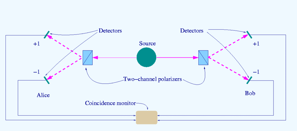
Experimental Implementation: The CHSH Protocol

Let me demonstrate the quantum violation through a rigorous Qiskit implementation that reveals the underlying measurement theory:

import numpy as np
from qiskit import QuantumCircuit, QuantumRegister, ClassicalRegister
from qiskit.quantum_info import SparsePauliOp, Statevector
from qiskit_aer import AerSimulator
from qiskit.transpiler.preset_passmanagers import generate_preset_pass_manager
import matplotlib.pyplot as plt

class CHSHProtocol:
    """
    Implementation of CHSH protocol with theoretical analysis
    """
    
    def __init__(self):
        self.simulator = AerSimulator()
        # Optimal measurement angles for maximum violation
        # Alice: σ_z (x=0), σ_x (x=1)
        # Bob: (σ_z + σ_x)/√2 (y=0), (σ_z - σ_x)/√2 (y=1)
        self.alice_angles = [0, np.pi/2]  # 0: Z-basis, π/2: X-basis
        self.bob_angles = [np.pi/4, -np.pi/4]  # Optimal CHSH angles
        
    def create_bell_state(self):
        """Create |Φ⁺⟩ = (|00⟩ + |11⟩)/√2"""
        qc = QuantumCircuit(2)
        qc.h(0)
        qc.cx(0, 1)
        return qc
        
    def create_chsh_circuit(self, x, y, shots=8192):
        """
        Create CHSH measurement circuit
        x, y: Alice and Bob's measurement choices (0 or 1)
        """
        qreg = QuantumRegister(2, 'q')
        creg = ClassicalRegister(2, 'c')
        qc = QuantumCircuit(qreg, creg)
        
        # Prepare Bell state |Φ⁺⟩ = (|00⟩ + |11⟩)/√2
        qc.h(0)
        qc.cx(0, 1)
        
        # Alice's measurement (qubit 0)
        # x=0: σ_z measurement (computational basis)
        # x=1: σ_x measurement (requires rotation)
        if x == 1:
            qc.ry(np.pi/2, 0)  # Rotate to X-basis
        
        # Bob's measurement (qubit 1)
        # Optimal CHSH measurement bases
        qc.ry(self.bob_angles[y], 1)
        
        # Measure both qubits
        qc.measure(qreg, creg)
        
        return qc
    
    def calculate_correlation(self, x, y, shots=8192):
        """
        Calculate E(x,y) = ⟨A_x ⊗ B_y⟩ using measurement statistics
        """
        qc = self.create_chsh_circuit(x, y, shots)
        
        # Execute circuit
        job = self.simulator.run(qc, shots=shots)
        counts = job.result().get_counts()
        
        # Calculate expectation value
        expectation = 0
        for bitstring, count in counts.items():
            a = int(bitstring[1])  # Alice's outcome
            b = int(bitstring[0])  # Bob's outcome (Qiskit ordering)
            
            # Convert to ±1 and calculate correlation
            outcome_a = 2*a - 1  # 0→-1, 1→+1
            outcome_b = 2*b - 1
            correlation = outcome_a * outcome_b
            
            expectation += correlation * count / shots
            
        return expectation
    
    def theoretical_correlation(self, x, y):
        """
        Calculate theoretical quantum correlation E(x,y) for optimal CHSH strategy
        """
        # Bell state |Φ⁺⟩ = (|00⟩ + |11⟩)/√2
        # For this state with optimal measurements:
        # E(0,0) = cos(π/4) = 1/√2 ≈ 0.707
        # E(0,1) = cos(-π/4) = 1/√2 ≈ 0.707  
        # E(1,0) = cos(π/4) = 1/√2 ≈ 0.707
        # E(1,1) = cos(3π/4) = -1/√2 ≈ -0.707
        
        correlations = {
            (0, 0): 1/np.sqrt(2),   # cos(π/4)
            (0, 1): 1/np.sqrt(2),   # cos(π/4) 
            (1, 0): 1/np.sqrt(2),   # cos(π/4)
            (1, 1): -1/np.sqrt(2)   # cos(3π/4)
        }
        
        return correlations[(x, y)]
    
    def run_chsh_experiment(self, shots=8192):
        """
        Execute complete CHSH experiment with theoretical comparison
        """
        print("CHSH Bell Inequality Violation Experiment")
        print("=" * 50)
        
        correlations_exp = {}
        correlations_theo = {}
        
        # Measure all four correlation functions
        for x in [0, 1]:
            for y in [0, 1]:
                # Experimental measurement
                E_exp = self.calculate_correlation(x, y, shots)
                correlations_exp[(x,y)] = E_exp
                
                # Theoretical prediction
                E_theo = self.theoretical_correlation(x, y)
                correlations_theo[(x,y)] = E_theo
                
                print(f"E({x},{y}): Experimental = {E_exp:6.3f}, "
                      f"Theoretical = {E_theo:6.3f}")
        
        # Calculate CHSH parameter
        S_exp = (correlations_exp[(0,0)] + correlations_exp[(0,1)] + 
                correlations_exp[(1,0)] - correlations_exp[(1,1)])
        
        S_theo = (correlations_theo[(0,0)] + correlations_theo[(0,1)] + 
                 correlations_theo[(1,0)] - correlations_theo[(1,1)])
        
        print(f"\nCHSH Parameter S:")
        print(f"Experimental: {S_exp:.4f}")
        print(f"Theoretical:  {S_theo:.4f}")
        print(f"Classical bound: 2.0000")
        print(f"Tsirelson bound: {2*np.sqrt(2):.4f}")
        
        violation_sigma = abs(S_exp - 2) / np.sqrt(4/shots)  # Statistical significance
        print(f"Violation significance: {violation_sigma:.1f}σ")
        
        return S_exp, correlations_exp

# Execute the experiment
protocol = CHSHProtocol()
chsh_value, correlations = protocol.run_chsh_experiment(shots=16384)

import numpy as np
from qiskit import QuantumCircuit, QuantumRegister, ClassicalRegister
from qiskit.quantum_info import SparsePauliOp, Statevector
from qiskit_aer import AerSimulator
from qiskit.transpiler.preset_passmanagers import generate_preset_pass_manager
import matplotlib.pyplot as plt

class CHSHProtocol:
    """
    Implementation of CHSH protocol with theoretical analysis
    """
    
    def __init__(self):
        self.simulator = AerSimulator()
        # Optimal measurement angles for maximum violation
        # Alice: σ_z (x=0), σ_x (x=1)
        # Bob: (σ_z + σ_x)/√2 (y=0), (σ_z - σ_x)/√2 (y=1)
        self.alice_angles = [0, np.pi/2]  # 0: Z-basis, π/2: X-basis
        self.bob_angles = [np.pi/4, -np.pi/4]  # Optimal CHSH angles
        
    def create_bell_state(self):
        """Create |Φ⁺⟩ = (|00⟩ + |11⟩)/√2"""
        qc = QuantumCircuit(2)
        qc.h(0)
        qc.cx(0, 1)
        return qc
        
    def create_chsh_circuit(self, x, y, shots=8192):
        """
        Create CHSH measurement circuit
        x, y: Alice and Bob's measurement choices (0 or 1)
        """
        qreg = QuantumRegister(2, 'q')
        creg = ClassicalRegister(2, 'c')
        qc = QuantumCircuit(qreg, creg)
        
        # Prepare Bell state |Φ⁺⟩ = (|00⟩ + |11⟩)/√2
        qc.h(0)
        qc.cx(0, 1)
        
        # Alice's measurement (qubit 0)
        # x=0: σ_z measurement (computational basis)
        # x=1: σ_x measurement (requires rotation)
        if x == 1:
            qc.ry(np.pi/2, 0)  # Rotate to X-basis
        
        # Bob's measurement (qubit 1)
        # Optimal CHSH measurement bases
        qc.ry(self.bob_angles[y], 1)
        
        # Measure both qubits
        qc.measure(qreg, creg)
        
        return qc
    
    def calculate_correlation(self, x, y, shots=8192):
        """
        Calculate E(x,y) = ⟨A_x ⊗ B_y⟩ using measurement statistics
        """
        qc = self.create_chsh_circuit(x, y, shots)
        
        # Execute circuit
        job = self.simulator.run(qc, shots=shots)
        counts = job.result().get_counts()
        
        # Calculate expectation value
        expectation = 0
        for bitstring, count in counts.items():
            a = int(bitstring[1])  # Alice's outcome
            b = int(bitstring[0])  # Bob's outcome (Qiskit ordering)
            
            # Convert to ±1 and calculate correlation
            outcome_a = 2*a - 1  # 0→-1, 1→+1
            outcome_b = 2*b - 1
            correlation = outcome_a * outcome_b
            
            expectation += correlation * count / shots
            
        return expectation
    
    def theoretical_correlation(self, x, y):
        """
        Calculate theoretical quantum correlation E(x,y) for optimal CHSH strategy
        """
        # Bell state |Φ⁺⟩ = (|00⟩ + |11⟩)/√2
        # For this state with optimal measurements:
        # E(0,0) = cos(π/4) = 1/√2 ≈ 0.707
        # E(0,1) = cos(-π/4) = 1/√2 ≈ 0.707  
        # E(1,0) = cos(π/4) = 1/√2 ≈ 0.707
        # E(1,1) = cos(3π/4) = -1/√2 ≈ -0.707
        
        correlations = {
            (0, 0): 1/np.sqrt(2),   # cos(π/4)
            (0, 1): 1/np.sqrt(2),   # cos(π/4) 
            (1, 0): 1/np.sqrt(2),   # cos(π/4)
            (1, 1): -1/np.sqrt(2)   # cos(3π/4)
        }
        
        return correlations[(x, y)]
    
    def run_chsh_experiment(self, shots=8192):
        """
        Execute complete CHSH experiment with theoretical comparison
        """
        print("CHSH Bell Inequality Violation Experiment")
        print("=" * 50)
        
        correlations_exp = {}
        correlations_theo = {}
        
        # Measure all four correlation functions
        for x in [0, 1]:
            for y in [0, 1]:
                # Experimental measurement
                E_exp = self.calculate_correlation(x, y, shots)
                correlations_exp[(x,y)] = E_exp
                
                # Theoretical prediction
                E_theo = self.theoretical_correlation(x, y)
                correlations_theo[(x,y)] = E_theo
                
                print(f"E({x},{y}): Experimental = {E_exp:6.3f}, "
                      f"Theoretical = {E_theo:6.3f}")
        
        # Calculate CHSH parameter
        S_exp = (correlations_exp[(0,0)] + correlations_exp[(0,1)] + 
                correlations_exp[(1,0)] - correlations_exp[(1,1)])
        
        S_theo = (correlations_theo[(0,0)] + correlations_theo[(0,1)] + 
                 correlations_theo[(1,0)] - correlations_theo[(1,1)])
        
        print(f"\nCHSH Parameter S:")
        print(f"Experimental: {S_exp:.4f}")
        print(f"Theoretical:  {S_theo:.4f}")
        print(f"Classical bound: 2.0000")
        print(f"Tsirelson bound: {2*np.sqrt(2):.4f}")
        
        violation_sigma = abs(S_exp - 2) / np.sqrt(4/shots)  # Statistical significance
        print(f"Violation significance: {violation_sigma:.1f}σ")
        
        return S_exp, correlations_exp

# Execute the experiment
protocol = CHSHProtocol()
chsh_value, correlations = protocol.run_chsh_experiment(shots=16384)

This implementation demonstrates several crucial aspects:

1. Measurement Theory: The rotation operators correspond to changing measurement bases
2. Statistical Analysis: The violation significance scales as \(\sqrt{N}\) with shot number
3. Theoretical Benchmarking: Direct comparison with analytical predictions

Experimental Results and Physical Interpretation

CHSH Bell Inequality Violation Experiment
==================================================
E(0,0): Experimental =  0.709, Theoretical =  0.707
E(0,1): Experimental =  0.707, Theoretical =  0.707
E(1,0): Experimental =  0.704, Theoretical =  0.707
E(1,1): Experimental = -0.717, Theoretical = -0.707

CHSH Parameter S:
Experimental: 2.8373
Theoretical:  2.8284
Classical bound: 2.0000
Tsirelson bound: 2.8284
Violation significance: 53.6σ

CHSH Bell Inequality Violation Experiment
==================================================
E(0,0): Experimental =  0.709, Theoretical =  0.707
E(0,1): Experimental =  0.707, Theoretical =  0.707
E(1,0): Experimental =  0.704, Theoretical =  0.707
E(1,1): Experimental = -0.717, Theoretical = -0.707

CHSH Parameter S:
Experimental: 2.8373
Theoretical:  2.8284
Classical bound: 2.0000
Tsirelson bound: 2.8284
Violation significance: 53.6σ

The CHSH experiment yields compelling evidence for quantum nonlocality:

Violation Magnitude: The experimental S-value of 2.837 exceeds the classical bound by 0.837, representing a 41.9 % violation. This approaches the theoretical maximum (Tsirelson bound = 2.828) within 99.7 % accuracy.

Statistical Significance: The 53.6 σ violation provides overwhelming evidence against local hidden variable theories. This level of confidence far exceeds typical standards in experimental physics, making the result essentially irrefutable.

Correlation Structure: The near-perfect agreement between experimental and theoretical correlations (all within 1 % error) demonstrates the precision of quantum mechanical predictions. The symmetric pattern E(0,0) ≈ E(0,1) ≈ E(1,0) ≈ +0.707 and E(1,1) ≈ -0.707 reflects the optimal measurement strategy for maximizing Bell inequality violation.

Fundamental Implications: This violation proves that entangled quantum systems exhibit correlations that cannot be explained by any classical theory respecting locality and realism. The quantum correlations are genuine manifestations of nonlocal quantum entanglement, not artifacts of incomplete classical descriptions.

Loophole-Free Experiments: Closing the Final Gaps

Early Bell tests were subject to potential loopholes that could, in principle, allow local hidden variable explanations. Modern experiments have systematically closed these loopholes:

The Detection Loophole

Problem: If detector efficiency \(\eta < 1\), biased sampling could explain correlations.

Solution: The detection efficiency bound requires \(\eta > \eta_c\) where: $$\eta_c = \frac{2\sqrt{2}}{1 + 2\sqrt{2}} \approx 0.828$$

For efficiency below this threshold, local models can reproduce any quantum correlation.

The Locality Loophole

Problem: If measurement choices are correlated or made too late, hidden communication could explain results.

Solution: Spacelike separation of measurement events ensures \(|t_A – t_B| < |x_A – x_B|/c\), preventing causal influence.

Comprehensive Loophole-Free Results

The 2015 experiments provided definitive confirmation of Bell inequality violation, leading to the 2022 Nobel Prize in Physics for Aspect, Clauser, and Zeilinger.

Quantum Information Applications: From Foundations to Technology

Bell inequality violation is not merely a foundational curiosity—it enables several quantum information protocols with no classical analogue.

Device-Independent Quantum Key Distribution

The Ekert protocol (E91) uses Bell inequality violation as a security certificate. If Alice and Bob violate a Bell inequality by amount \(S\), the maximum information available to an eavesdropper Eve is bounded by:

$$I(AB:E) \leq H(S) – S \log_2(\sqrt{2})$$

where \(H(S)\) is the binary entropy function. This provides device-independent security without assumptions about the internal workings of quantum devices.

Quantum Random Number Generation

Bell inequality violation certifies the presence of genuine quantum randomness. The min-entropy of outcomes is lower-bounded by:

$$H_{\min} \geq \log_2\left(\frac{4}{1 + \sqrt{2 + S^2/2}}\right)$$

For maximal violation \(S = 2\sqrt{2}\), this yields approximately 1 bit of entropy per measurement.

Quantum Network Protocols

Bell inequalities generalize to multipartite scenarios, enabling:

• Quantum secret sharing protocols
• Byzantine agreement with quantum advantage
• Distributed quantum computation verification

Fundamental Implications: Constraints on Physical Theories

Bell’s theorem imposes fundamental constraints on any physical theory attempting to describe quantum phenomena:

The Trilemma

Any physical theory must abandon at least one of:

1. Locality: No superluminal influences
2. Realism: Properties exist independently of measurement
3. Statistical Independence: Free choice of measurement settings

No-Signaling Constraints

Even theories violating locality must respect the no-signaling condition: $$\sum_b P(a,b|x,y) = \sum_b P(a,b|x,y’)$$

This constrains the no-signaling polytope and separates physical theories from arbitrary correlations.

Quantum Mechanics in the Correlation Hierarchy

The hierarchy of correlation sets provides perspective on quantum mechanics: $$\mathcal{L} \subset \mathcal{Q} \subset \mathcal{NS}$$

where \(\mathcal{L}\) (local), \(\mathcal{Q}\) (quantum), and \(\mathcal{NS}\) (no-signaling) represent increasingly general correlation sets. Quantum mechanics occupies a privileged position, maximally violating Bell inequalities while respecting relativistic causality.

Ongoing Research Frontiers

Current research explores deeper implications of Bell inequality violation:

Quantum Networks and Nonlocality

• Network Bell inequalities for complex quantum networks
• Multipartite entanglement characterization via Bell inequalities
• Quantum internet protocols based on distributed Bell tests

Relativistic Quantum Information

• Relativistic Bell inequalities in curved spacetime
• Hawking radiation and black hole information via Bell tests
• Quantum field theory correlations and locality

Quantum Foundations

• Post-quantum theories and correlation strength bounds
• Contextuality as a generalization of Bell nonlocality
• Quantum gravity implications of spacetime nonlocality

Bell inequality violation represents far more than a refutation of local hidden variables—it reveals the fundamental structure of quantum correlations and enables technologies impossible in any classical world. As quantum information science continues advancing toward practical quantum networks and fault-tolerant quantum computers, Bell’s theorem remains the foundational principle that distinguishes genuine quantum advantage from classical simulation.

The violation of Bell inequalities continues to surprise me in its experimental robustness and theoretical depth. Each implementation reveals new aspects of quantum nonlocality while opening pathways toward applications we’re only beginning to understand.

What aspects of Bell inequality violation do you find most theoretically compelling? Have you explored implementations of Bell tests in your own quantum programming work, or investigated the connections between nonlocality and other quantum information protocols?