Bell States Quantum Theory: Mathematical Foundation and Structure
In our previous post, we successfully created and measured bell states quantum circuits using Qiskit. We wrote code that generated the state \(|\Phi^+\rangle = \frac{1}{\sqrt{2}}(|00\rangle + |11\rangle)\), observed the characteristic 50-50 measurement distribution, and witnessed quantum entanglement in action.
But what exactly did we create? Why are bell states quantum systems considered the cornerstone of quantum information theory?
Key Question: These seemingly simple quantum states revolutionized our understanding of reality and became the foundation for quantum computing, cryptography, and communication protocols.
Today, we dive deep into the mathematical structure and physical significance of bell states quantum mechanics, exploring the elegant mathematical framework that makes quantum entanglement possible.
Understanding Bell States Quantum Mechanics in Hilbert Space
The Mathematical Playground: Complex Vector Spaces
Bell states quantum systems operate within complex vector spaces called Hilbert spaces. Think of these as the mathematical “playground” where all quantum phenomena occur.
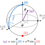
For a single qubit, this space is \(\mathcal{H} = \mathbb{C}^2\), spanned by the computational basis \({|0\rangle, |1\rangle}\). Any single-qubit state can be written as:
$$ |\psi\rangle = \alpha|0\rangle + \beta|1\rangle$$
where \(\alpha, \beta \in \mathbb{C}\) satisfy the normalization condition \(|\alpha|^2 + |\beta|^2 = 1\).
For bell states quantum systems, we work in the tensor product space \(\mathcal{H} \otimes \mathcal{H} = \mathbb{C}^4\), with computational basis:
| State | Tensor Product Form | Binary Representation |
|---|---|---|
| \(|00\rangle\) | \(|0\rangle_A \otimes |0\rangle_B\) | Both qubits in 0 |
| \(|01\rangle\) | \(|0\rangle_A \otimes |1\rangle_B\) | First 0, second 1 |
| \(|10\rangle\) | \(|1\rangle_A \otimes |0\rangle_B\) | First 1, second 0 |
| \(|11\rangle\) | \(|1\rangle_A \otimes |1\rangle_B\) | Both qubits in 1 |
Quantum Entanglement Theory: The Heart of the Mystery
Separable vs Entangled States
Mathematical Definition of Entanglement
The crucial distinction in quantum entanglement theory lies between separable and entangled states. A two-qubit state is separable if it can be written as a tensor product:
$\(|\psi\rangle = |\phi\rangle_A \otimes |\phi\rangle_B\)$
If no such decomposition exists, the state is entangled.
Example of Separable State: $\(|\psi_{\text{sep}}\rangle = \frac{1}{\sqrt{2}}(|0\rangle + |1\rangle)_A \otimes |0\rangle_B = \frac{1}{\sqrt{2}}(|00\rangle + |10\rangle)\)$
Example of Entangled State (Bell State): $\(|\psi_{\text{ent}}\rangle = \frac{1}{\sqrt{2}}(|00\rangle + |11\rangle)\)$
This cannot be written as a product of individual qubit states!
This mathematical property has profound physical implications: entangled systems cannot be described independently, even when spatially separated—the hallmark of bell states quantum mechanics.
Einstein’s Concern: “Spooky action at a distance” was Einstein’s dismissive term for quantum entanglement. He couldn’t accept that measurement on one particle could instantly affect another, regardless of distance.
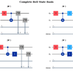
Bell States Quantum Systems: Four Fundamental Entangled States
The Complete Bell Basis
Bell states quantum mechanics defines four maximally entangled states that form a complete orthogonal basis for the two-qubit Hilbert space:
 The Four Bell States:

|Φ⁺⟩ = (1/√2)(|00⟩ + |11⟩)  ← We created this one!
|Φ⁻⟩ = (1/√2)(|00⟩ - |11⟩)
|Ψ⁺⟩ = (1/√2)(|01⟩ + |10⟩)
|Ψ⁻⟩ = (1/√2)(|01⟩ - |10⟩)
These bell states quantum systems exhibit perfect correlations: measuring one qubit instantly determines the measurement outcome of its entangled partner, regardless of spatial separation.
Circuit Generation of Bell States
The standard circuit for generating bell states quantum systems uses two fundamental gates:
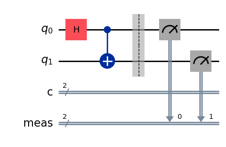
- CNOT Gate: Creates conditional entanglement
- Hadamard Gate (H): Creates superposition on first qubit
Step-by-step transformation: $$|00\rangle \rightarrow \frac{1}{\sqrt{2}}(|00\rangle + |10\rangle) \rightarrow \frac{1}{\sqrt{2}}(|00\rangle + |11\rangle)$$
Mathematical Properties: Orthogonality and Completeness
The bell states quantum basis satisfies crucial mathematical properties:
Orthonormality Proof
Mathematical Verification
Orthogonality Example: \(\langle\Phi^+|\Phi^-\rangle = \frac{1}{2}(\langle00| + \langle11|)(|00\rangle – |11\rangle) = \frac{1}{2}(1 – 1) = 0\)
Normalization: \(\langle\Phi^+|\Phi^+\rangle = \frac{1}{2}(\langle00| + \langle11|)(|00\rangle + |11\rangle) = \frac{1}{2}(1 + 1) = 1\)
Completeness Relation: \(\sum_{i} |\text{Bell}_i\rangle\langle\text{Bell}_i| = I_4\)
This orthogonality means any two-qubit state can be expanded in the bell states quantum basis:
\(|\psi\rangle = c_1|\Phi^+\rangle + c_2|\Phi^-\rangle + c_3|\Psi^+\rangle + c_4|\Psi^-\rangle\)
Quantum Insight: Just as any vector in 3D space can be written as a combination of x̂, ŷ, ẑ unit vectors, any two-qubit quantum state can be written as a combination of the four Bell states.
Schmidt Decomposition in Bell States Quantum Analysis
Schmidt Decomposition Quantum Theory: The Universal Tool
For any bipartite pure state \(|\psi\rangle_{AB}\), the schmidt decomposition quantum formalism provides the most elegant way to analyze entanglement:
\(|\psi\rangle_{AB} = \sum_{i=0}^{r-1} \sqrt{\lambda_i}|u_i\rangle_A \otimes |v_i\rangle_B\)
Where:
- \({|u_i\rangle_A}\) and \({|v_i\rangle_B}\) are orthonormal bases
- \(\lambda_i > 0\) are the Schmidt coefficients
- \(r\) is the Schmidt rank
Bell States Analysis Using Schmidt Decomposition
Example: Analyzing \(|\Phi^+\rangle\)
The bell states quantum system \(|\Phi^+\rangle = \frac{1}{\sqrt{2}}(|00\rangle + |11\rangle)\) is already in Schmidt form:
$$ |\Phi^+\rangle = \frac{1}{\sqrt{2}}|0\rangle_A \otimes |0\rangle_B + \frac{1}{\sqrt{2}}|1\rangle_A \otimes |1\rangle_B$$
Schmidt Analysis Results:
| Property | Value | Interpretation |
|---|---|---|
| Schmidt Coefficients | \(\lambda_0 = \lambda_1 = \frac{1}{2}\) | Equal weights |
| Schmidt Rank | \(r = 2\) | Maximum for 2-qubit system |
| Entanglement | Maximal | Cannot be more entangled |
Density Matrix Representation
In the density matrix formalism, bell states quantum systems reveal their structure through off-diagonal terms:
$$ \rho_{\Phi^+} = |\Phi^+\rangle\langle\Phi^+| = \frac{1}{2}\begin{pmatrix} 1 & 0 & 0 & 1 \ 0 & 0 & 0 & 0 \ 0 & 0 & 0 & 0 \ 1 & 0 & 0 & 1 \end{pmatrix}$$
Key Insight: The off-diagonal terms (1,4) and (4,1) capture the quantum coherence responsible for entanglement. If these terms decay (due to decoherence), entanglement is lost.
Entanglement Quantification: Measuring the Unmeasurable
Von Neumann Entropy: The Gold Standard
The entanglement entropy quantifies how much information is “hidden” in correlations between subsystems.
Calculation for Bell States:
Entropy Calculation
Step-by-step Calculation
Reduced density matrix for subsystem A: $\(\rho_A = \text{Tr}B(\rho{AB}) = \frac{1}{2}(|0\rangle\langle0| + |1\rangle\langle1|) = \frac{I}{2}\)$
Eigenvalues: \(\lambda_1 = \lambda_2 = \frac{1}{2}\)
Von Neumann entropy: $\(S(\rho_A) = -\text{Tr}(\rho_A \log_2 \rho_A) = -\frac{1}{2}\log_2\frac{1}{2} – \frac{1}{2}\log_2\frac{1}{2} = 1\)$
Result: \(S = 1\) ebit (maximum possible for two qubits)
Entanglement Hierarchy:

Separable States:     S = 0 ebits  (no entanglement)
Partially Entangled:  0 < S < 1    (some entanglement)
Bell States:          S = 1 ebit   (maximum entanglement)
Concurrence: An Alternative Measure
For mixed states, concurrence provides another entanglement quantification:
$$ C(\rho) = \max{0, \sqrt{\lambda_1} – \sqrt{\lambda_2} – \sqrt{\lambda_3} – \sqrt{\lambda_4}}$$
For pure bell states quantum systems: \(C = 1\) (maximal entanglement)
Physical Implementations: From Theory to Reality
Hardware Platforms for Bell States Generation
Different quantum computing platforms generate bell states quantum systems through various physical mechanisms:
| Platform | Mechanism | Typical Fidelity | Companies |
|---|---|---|---|
| Superconducting | Microwave pulses | 99.5%+ | IBM, Google, Rigetti |
| Trapped Ions | Laser manipulation | 99.9%+ | IonQ, Alpine Quantum |
| Photonic | Beam splitters | 95%+ | Xanadu, PsiQuantum |
| Silicon Dots | Electric field control | 99%+ | Intel, SiQURE |
Experimental Challenges
Reality Check: While mathematically perfect, real bell states quantum systems face decoherence, gate errors, and measurement noise. Current quantum computers achieve Bell state fidelities of 95-99.9%, depending on the platform.
Common Error Sources
Decoherence: Environmental interactions destroy quantum coherence
T₁ (relaxation): Energy decay to ground state
T₂ (dephasing): Phase relationship decay
Gate Errors: Imperfect implementation of H and CNOT gates
Calibration drift
Crosstalk between qubits
Measurement Errors: Incorrect state classification
SPAM errors (State Preparation and Measurement)
Readout fidelity typically 95-99%
Connecting to Quantum Information Theory
Bell states quantum theory serves as the foundation for numerous quantum information protocols:
Applications Preview:

• Quantum Teleportation    → Transfer quantum states
• Quantum Cryptography     → Unbreakable security
• Quantum Error Correction → Protect quantum information
• Quantum Computing        → Universal gate sets
In our next post, we’ll explore how bell states quantum correlations violate classical physics through Bell’s theorem, leading to groundbreaking experiments that earned the 2022 Nobel Prize in Physics.
Summary: The Mathematical Beauty of Quantum Entanglement
Bell states quantum theory demonstrates the elegant mathematical structure underlying quantum mechanics:
- Hilbert Space Framework: Complex vector spaces enable superposition and entanglement
- Schmidt Decomposition: Provides optimal entanglement analysis tool
- Maximal Entanglement: Bell states achieve maximum possible two-qubit entanglement
- Perfect Correlations: Measurement outcomes are 100% correlated despite spatial separation
Final Thought: The mathematical formalism of bell states quantum mechanics is more than abstract theory—it’s the blueprint for quantum technologies that will transform computing, communication, and cryptography in the coming decades.
Next Up: “Bell Theorem Inequality Violation: From EPR Paradox to Quantum Information” – where we’ll see how these mathematical constructs challenge our fundamental understanding of reality itself.