Linear Algebra for Quantum Computing: The Mathematical Foundation You Need
When I first encountered quantum computing during my physics undergraduate studies, I wondered: “Why do I need to understand linear algebra again?” As a physics student, I had already struggled through vector calculus and matrix operations for classical mechanics and electromagnetism. But quantum computing demanded something different – not just computational skills, but a deep understanding of why mathematics shapes the quantum world itself.
“The mathematics is not there till we put it there.” – Arthur Eddington
Today, I want to share what I’ve learned about why linear algebra isn’t just a prerequisite for quantum computing – it’s the language quantum states speak. This is the beginning of my journey into quantum computing fundamentals, and I hope you’ll join me as we explore these concepts together.
Why Classical Bits Are Not Enough
Let’s start with what we know. In classical computing, information is stored in bits that can be either 0 or 1. Simple, binary, definitive. When we want to represent the state of a classical bit mathematically, we might write:
Bit state: 0 or 1
Mathematical representation: {0, 1}
But here’s where quantum computing becomes fascinating: quantum bits (qubits) can exist in what we call superposition– they can be in a combination of both 0 and 1 states simultaneously. This isn’t just a quirky quantum property; it’s the fundamental reason quantum computers can potentially solve certain problems exponentially faster than classical computers.
To represent this mathematically, we need something more sophisticated than simple binary notation. We need vectors.
Vectors as Quantum States
In quantum computing, we represent the state of a qubit using a state vector in a 2-dimensional complex vector space. The two basis states |0⟩ and |1⟩ (read as “ket zero” and “ket one” in Dirac notation) correspond to our classical bit states, but now we can have linear combinations:
|ψ⟩ = α|0⟩ + β|1⟩
Where α and β are complex numbers called probability amplitudes, and |ψ⟩ (read as “psi”) represents our quantum state.
Let me show you this with a practical example using Qiskit:
import numpy as np
from qiskit import QuantumCircuit, Aer, execute
from qiskit.quantum_info import Statevector

# Create a simple quantum state vector
# This represents a qubit in equal superposition
statevector = Statevector([1/np.sqrt(2), 1/np.sqrt(2)])
print("State vector:", statevector)
print("Probabilities:", statevector.probabilities())
When you run this code, you’ll see that our qubit is in a state where measuring it gives us a 50% chance of finding it in state |0⟩ and a 50% chance of finding it in state |1⟩.
Why vectors matter: Vectors give us the mathematical framework to represent not just the “what” (the measurement outcomes) but also the “how much” (the probability amplitudes) of quantum states.
The Normalization Constraint
Here’s a crucial mathematical requirement that connects linear algebra to quantum physics: the state vector must be normalized. This means:
|α|² + |β|² = 1
This constraint ensures that the total probability of finding the qubit in any possible state equals 100%. It’s not just a mathematical convenience – it’s a fundamental requirement of quantum mechanics.<details> <summary><strong>Mathematical Proof: Why Unit Vectors?</strong></summary>
The normalization condition comes from the Born rule, which states that the probability of measuring a quantum system in a particular state is given by the square of the absolute value of the probability amplitude.
For a qubit in state |ψ⟩ = α|0⟩ + β|1⟩:
- Probability of measuring |0⟩ = |α|²
- Probability of measuring |1⟩ = |β|²
Since these are the only two possible outcomes, and probabilities must sum to 1: |α|² + |β|² = 1
This mathematical constraint reflects the physical reality that something must be observed when we measure a quantum system.</details>
Inner Products and Quantum Probabilities
The inner product (also called dot product) in quantum mechanics has a special physical meaning. For two quantum states |ψ⟩ and |φ⟩, the inner product ⟨φ|ψ⟩ gives us the probability amplitude for transitioning from state |ψ⟩ to state |φ⟩.
The probability of this transition is:
P(φ|ψ) = |⟨φ|ψ⟩|²
Let’s see this in action:
# Create two different quantum states
state1 = Statevector([1, 0])  # |0⟩ state
state2 = Statevector([1/np.sqrt(2), 1/np.sqrt(2)])  # Equal superposition

# Calculate the inner product
inner_product = state1.inner(state2)
probability = abs(inner_product)**2

print(f"Inner product: {inner_product}")
print(f"Transition probability: {probability}")
This will show you that there’s a 50% probability of measuring the superposition state and finding it in the |0⟩ state.
Your First Quantum State with Qiskit
Now let’s create and manipulate our first quantum state using Qiskit:
from qiskit import QuantumCircuit, ClassicalRegister, QuantumRegister
from qiskit.visualization import plot_histogram
import matplotlib.pyplot as plt

# Create a quantum circuit with 1 qubit and 1 classical bit
qc = QuantumCircuit(1, 1)

# Apply a Hadamard gate to create superposition
# This puts our qubit in the state (|0⟩ + |1⟩)/√2
qc.h(0)

# Measure the qubit
qc.measure(0, 0)

# Execute the circuit
backend = Aer.get_backend('qasm_simulator')
job = execute(qc, backend, shots=1000)
result = job.result()
counts = result.get_counts(qc)

print("Measurement results:", counts)
plot_histogram(counts)
plt.show()
When you run this code multiple times, you’ll see approximately 50% of measurements yielding 0 and 50% yielding 1, confirming our mathematical prediction.
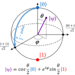
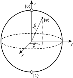
The Bloch Sphere: Visualizing Qubit States
Every single qubit state can be visualized on what we call the Bloch sphere – a 3D representation where:
- The north pole represents |0⟩
- The south pole represents |1⟩
- Points on the equator represent various superposition states
- The radius is always 1 (because our state vectors are normalized)
from qiskit.visualization import plot_bloch_vector

# Visualize the |0⟩ state
plot_bloch_vector([0, 0, 1], title="State |0⟩")

# Visualize the equal superposition state
plot_bloch_vector([1, 0, 0], title="Superposition State")
This geometric interpretation helps us understand why linear algebra is so natural for quantum computing – quantum states literally live in vector spaces!
Why This Mathematical Foundation Matters
Understanding these linear algebra concepts isn’t just academic exercise. Here’s why they’re crucial:
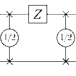
- Quantum Gates are Matrices: Every operation we perform on qubits corresponds to multiplying our state vector by a matrix
- Quantum Algorithms: Complex quantum algorithms like Shor’s and Grover’s are built on these mathematical foundations
- Error Correction: Quantum error correction relies heavily on linear algebra concepts
- Quantum Machine Learning: The intersection of quantum computing and AI is fundamentally mathematical
What’s Coming Next
In our next post, we’ll dive into complex numbers in quantum mechanics – why quantum states need complex probability amplitudes and how this connects to the wave-like nature of quantum systems. We’ll also explore:
- The role of phase in quantum computing
- Why global phase doesn’t matter but relative phase does
- Practical examples with Qiskit
Your homework: Try running the code examples above and experiment with different state vectors. What happens when you create a state vector [0.8, 0.6]? What about [1, 1]? (Hint: one of these won’t work – can you figure out why?)
This is the first post in my quantum computing fundamentals series. I’m learning these concepts alongside writing about them, so if you spot any errors or have insights to share, please let me know in the comments. You can also read about my background and why I started this magazine in my previous posts.
References and Further Reading:
- IBM Qiskit Textbook – Linear Algebra
- Nielsen, M. A., & Chuang, I. L. (2010). Quantum Computation and Quantum Information
- Microsoft Quantum Development Kit Documentation